
Beyond Backup: A Deep Dive into EBS Snapshots 💾
A Deep Dive into Incremental Mechanics, Restore Performance, and Billing Strategy

In cloud architecture, Amazon EBS Snapshots are often relegated to the simple category of “backups.” This is a profound understatement. In reality, they are a foundational AWS service that underpins data protection, disaster recovery, application scaling, and data migration.
Understanding the sophisticated, block-level engineering behind snapshots is essential for any professional building resilient, high-performance, and cost-effective systems on AWS.
This post will deconstruct the core mechanics of EBS Snapshots, their performance implications during restoration, and their strategic use in a multi-region architecture.
The Core Mechanic: True Incrementalism Explained ⛓️
The genius of EBS Snapshots lies in their point-in-time, incremental nature. This design is what makes them extraordinarily fast to create and efficient to store.
Here is a detailed breakdown of the process:
The First Snapshot (The Baseline): When you initiate the first snapshot of an EBS volume, AWS asynchronously copies all data blocks that have been written to (not the full provisioned size of the volume) to a secure, highly durable backend in Amazon S3. This first snapshot is the full baseline of your data at that exact moment.
Subsequent Snapshots (The Deltas): For every snapshot taken after the first, AWS only identifies and copies the data blocks that have changed since the last snapshot was taken. This “delta” is all that is saved.
A common professional analogy is to think of snapshots like Git commits.
The first snapshot is the initial commit of a full project.
Every subsequent snapshot is a new commit that only stores the diff (the changes).
When you restore any snapshot, AWS gives you the full “checked-out” version of your volume at that point in time, just as
git checkout <commit-hash>gives you the full state of your code.
Analogy: The Ever-Evolving Library 📚
To further clarify this crucial concept, let’s use an analogy of a highly efficient, version-controlled library:
Imagine your EBS volume is a vast library filled with books.
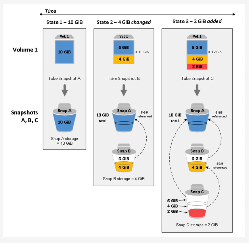
Taking the First Snapshot (Snap A): You decide to make a complete “inventory” of your library on Monday. This is your first snapshot. You meticulously list every book on every shelf, noting its contents. This comprehensive list (the full copy of written blocks) is stored safely in a central archive (S3).
Taking a Second Snapshot (Snap B): On Tuesday, you add a few new books and revise some existing ones. Instead of re-listing every single book in the entire library, you simply note down “Today, these specific new books were added, and these specific existing books had pages updated.” This “notes-only” approach is your second snapshot. It only records the changes (the incremental data). It knows to refer back to Monday’s inventory for all the other books that haven’t changed.
Taking a Third Snapshot (Snap C): On Wednesday, more changes occur. Again, you just note down the specific additions and revisions made since Tuesday. This is your third, even smaller, incremental snapshot.
The snapshot chain perfectly illustrates this. Snapshot A is the full 10 GiB. Snapshot B only stores the 4 GiB of changes. Snapshot C only stores the 2 GiB of new additions, leveraging the prior snapshots for the unchanged data.
The “Chain” and Deletion Mechanics
When you have a series of snapshots (e.g., Snap A -> Snap B -> Snap C), you have created a lineage. Snap C references blocks from Snap B, which in turn references blocks from Snap A.
A common misconception surrounds deletion. What happens if you delete Snap B, which is in the middle of the chain?
The chain does not break. The data is not “merged” in the way you might think. Instead, the snapshot system is intelligent. When you command a deletion of Snap B, the snapshot service identifies any unique data blocks that only Snap B stored but are still required by Snap C. Those specific blocks are preserved and their reference is “passed” to Snap C. Any blocks unique to Snap B that are not needed by any other snapshot are then marked for garbage collection and deleted.
Key takeaway: You can delete any snapshot in a lineage (except the last) with absolute safety. You will never lose data integrity for your other snapshots.
Performance Deep Dive: The Restore Process 🚀
Creating a snapshot is fast, but the restore process has critical performance implications that every architect must understand.
The “Lazy Load” Performance Penalty
When you create a new EBS volume from a snapshot, the AWS control plane returns a “success” message almost instantly. The volume appears in your console as available, and you can attach it to an EC2 instance.
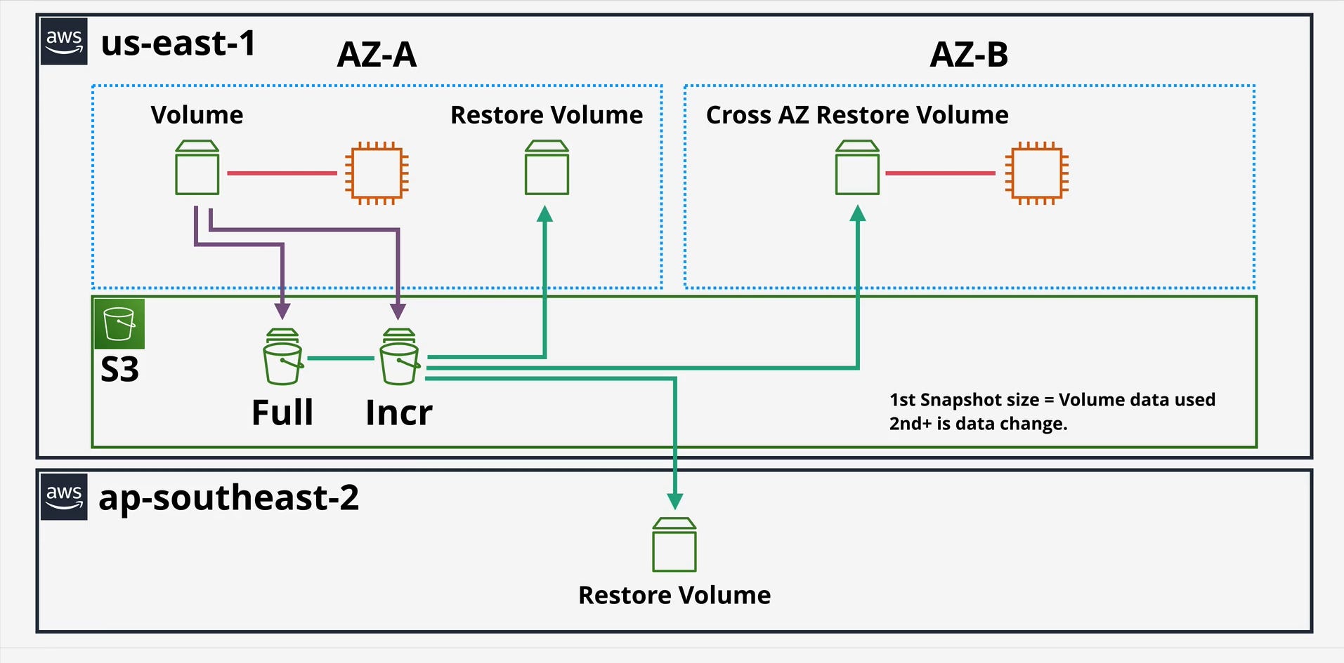
However, this is an abstraction. In the background, the volume is “lazy loading” its data. The data blocks are not all present on the new volume; they are being asynchronously hydrated (copied) from the snapshot’s storage in S3 on demand. Your high-level diagram shows this with the “Restore Volume” connecting back to S3.
This means the very first time your operating system or application attempts to read a specific block, it incurs a significant I/O latency penalty as that block is pulled from S3.
For I/O-intensive workloads, this is a major problem:
Database Servers: A newly restored database may be extremely slow as it performs index scans, forcing thousands of blocks to be lazy-loaded.
Boot Volumes: An instance booting from a custom AMI (which is backed by a snapshot) may take many minutes to become responsive as the OS files are read for the first time.
The legacy solution was “pre-warming”—a brute-force method where engineers would attach the new volume and run a utility (like dd or fio) to manually read every single block, forcing the full hydration before placing the volume in production. This is operationally complex and slow.
The Solution: Fast Snapshot Restore (FSR)
To solve this problem, AWS introduced Fast Snapshot Restore (FSR).
FSR is a feature you enable on a per-snapshot, per-Availability Zone (AZ) basis. When enabled, AWS maintains a fully hydrated, “hot” pool of data for that snapshot.
When you create a volume from an FSR-enabled snapshot (in the same AZ where FSR is enabled), the volume is fully initialized at creation. There is no lazy loading and no first-hit performance penalty. The volume instantly delivers its full provisioned IOPS and throughput.
Mechanically, FSR works on a credit-based system. Enabling FSR on a snapshot (e.g., a 1TiB snapshot) gives you a volume creation credit bucket. Creating one 1TiB volume from it consumes one credit. This credit bucket replenishes over time, allowing you to create multiple high-performance volumes.
Key takeaway: For any workload that is sensitive to restore latency (like auto-scaling groups with custom AMIs or rapid database failover), FSR is an essential, game-changing feature.
Global Architecture: Regional Features 🌎
EBS Snapshots are, by default, stored within the same AWS Region as the source volume. However, their strategic value is fully unlocked by their regional capabilities.
Cross-Region Copy (CRC)
You can copy any EBS snapshot from one AWS Region to another. This is the foundation of a robust disaster recovery (DR) strategy. Your first image clearly illustrates this with the arrow going from the S3 storage in us-east-1 down to ap-southeast-2 to create a “Restore Volume.”
Mechanics: The first time you copy a snapshot of a volume to a new region, it is a full copy of the snapshot’s data. Subsequent copies of snapshots from the same volume lineage to that same destination region are incremental.
Use Case: Disaster Recovery: CRC is the primary tool for achieving your Recovery Point Objective (RPO). By automating snapshot copies to a DR region, you ensure that you have a recent copy of your data (e.g., a 1-hour RPO) safe from a regional-level disaster.
Use Case: Migration & Sovereignty: CRC is the simplest way to migrate an application to a new region or to move data to a specific geography to comply with data sovereignty regulations.
AMIs and Snapshots
It is crucial to understand that an Amazon Machine Image (AMI) is not a single object. An AMI is a metadata pointer that references one or more EBS snapshots (one for the root volume and one for each attached data volume).
When you copy an AMI to another region, what you are actually doing under the hood is initiating a Cross-Region Copy job for its backing EBS snapshot(s).
Pro-Tip: To achieve the fastest Recovery Time Objective (RTO) in a DR scenario, you would combine these features:
Automate Cross-Region Copy (CRC) of your AMI and data snapshots to your DR region.
Enable Fast Snapshot Restore (FSR) on those copied snapshots in your DR region.
This ensures that in a disaster, you can instantly launch new instances from your AMI that are fully initialized and ready to handle production traffic immediately.
EBS Snapshots are a sophisticated, multi-faceted service. Mastering their incremental lineage allows you to manage data protection efficiently. Understanding their restore-time performance (Lazy Loading vs. FSR) is the key to building high-availability systems. And leveraging their regional capabilities is the cornerstone of a modern disaster recovery and global migration strategy.
EBS Snapshot Consumption and Billing 💰
Understanding the billing model for EBS Snapshots is as critical as understanding their technical function. The cost is not based on the provisioned size of your volumes, but on the actual data consumed by the snapshots. This model is built on two primary storage tiers and supplemented by costs for advanced features and data movement.
Here is a detailed breakdown.
1. The Core Billing Model: Storage Tiers
You are billed for where your snapshots are stored, which is divided into two main tiers.
EBS Snapshot Standard Tier (The “Hot” Tier)
This is the default, high-performance tier intended for snapshots you may need to access frequently, such as for daily backups, testing, or development.
How Consumption is Calculated: You are billed only for the unique, incremental data blocks your snapshot chain consumes.
Example:
You have a 100 GiB volume with 40 GiB of data.
Snap A (Monday): This first snapshot is a full copy of the written data. Your billable consumption is 40 GiB.
Snap B (Tuesday): You modify 5 GiB of data. This snapshot only stores those 5 GiB of changed blocks.
Snap C (Wednesday): You add 10 GiB of new data. This snapshot only stores those 10 GiB of new blocks.
Total Billable Storage: Your total consumption is not 100+100+100, nor is it 40+45+55. It is the sum of the unique blocks: 40 GiB (from A) + 5 GiB (from B) + 10 GiB (from C) = 55 GiB.
Deletion: If you delete Snap B, any of its 5 GiB of data that is still needed by Snap C is simply retained, and its cost is “passed” to Snap C. You are always just paying for the 55 GiB of unique data, regardless of how many or which snapshots you delete from the middle of the chain.
Billing: Billed per GiB-month (e.g., $0.05 per GiB-month in
us-east-1).Restores: Restoring a volume from the Standard tier is free.
EBS Snapshot Archive Tier (The “Cold” Tier) 🧊
This is a low-cost storage tier designed for long-term retention (months or years) where you do not expect to need fast or frequent access. This is ideal for compliance or end-of-project archival.
How Consumption is Calculated: When you “archive” a snapshot, AWS converts the incremental snapshot into a full, point-in-time snapshot and moves it to this tier. You are billed for the full size of that snapshot.
Example: If your volume had 60 GiB of data at the time of the snapshot, archiving it will store 60 GiB in the Archive tier, regardless of what other incremental snapshots exist.
Billing: Billed at a much lower GiB-month rate (e.g., $0.0125 per GiB-month, a 75% saving).
Key Caveats:
Minimum Retention: There is a 90-day minimum retention period. If you delete an archived snapshot after 60 days, you are still billed for the remaining 30 days.
Retrieval Cost: Restoring is not free. You pay a per-GiB retrieval fee (e.g., $0.03 per GiB) to move the snapshot from the Archive tier back to the Standard tier.
Retrieval Time: Restores are not instant. Retrieval from the Archive tier can take up to 72 hours.
2. Additional Cost Factors: Features and Data Movement
Beyond pure storage, you can incur costs from using specific features or moving data.
Fast Snapshot Restore (FSR)
This is the feature you enable to eliminate the “lazy loading” performance penalty. Because AWS is keeping a “hot,” fully initialized copy of your snapshot ready, this service incurs a separate charge.
How Consumption is Calculated: You are billed in Data Services Unit-Hours (DSU-Hours).
Billing: This is a separate, hourly charge per snapshot, per Availability Zone that it is enabled in.
Use Case: This cost is typically only justified for business-critical AMIs (like in an auto-scaling group) or database snapshots where instant, high-performance restore is a firm requirement (a low RTO).
Cross-Region Copy (CRC)
When you copy a snapshot to another region for disaster recovery, two types of costs are incurred:
Data Transfer: You pay a one-time “Data Transfer OUT” fee from the source region (e.g., from
us-east-1). Data transfer into the destination region (e.g.,eu-west-1) is free. This fee is billed per GiB transferred.Storage: Once the snapshot copy exists in the new region (
eu-west-1), it consumes storage just like any other snapshot in that region (at that region’s GiB-month rate). Remember, the first copy to a new region is a full copy, and subsequent copies are incremental.

Summary: Your Total Snapshot Bill
Your total monthly bill for EBS Snapshots is a combination of these components:
Standard Storage: (Total unique GiB in Standard tier) x (Standard GiB-month price)
Archive Storage: (Total full GiB in Archive tier) x (Archive GiB-month price)
Archive Retrievals: (Total GiB retrieved from Archive) x (Per-GiB retrieval price)
FSR Charges: (Total DSU-Hours used) x (DSU-Hour price)
Data Transfer: (Total GiB copied to other regions) x (Data Transfer OUT price)